Playtime: explorations with OpenAI’s GPT-4, introduction

Featured

I will be honest. I have been very busy and unable to write much. Specifically on the latest advances in large language models and their applications, I had forced myself to stay on the fence. Yes, read about it, stay on top of the developments, but leave the experimenting to others, for the time being. Then two things changed my mind: first, I started working through David Mertz’ book Regular Expression Puzzles and AI Coding Assistants (very superficially, admittedly, as regular expressions are not my forte, but the book is awesome); second, I chanced on the article Why everyone should try GPT-4, even the CEO by Cassie Kozyrkov.

Here are the things I am actively playing with, right now. Soon I will start documenting these explorations with a new series of short blog posts:

  • Writing an essay in philosophy based on a specific, complex prompt
  • Act as baking assistant 
  • Write an imaginary dialogue between specific historic and fictional characters
  • Demonstrate geometry theorem
  • Perform arithmetic operations 
  • Act as song translation assistant
  • Write poem with specific metric, and music in a specific composer’s style
  • Act as coding assistant
  • Solve puzzles 
  • Play a live tic tac toe and/or chess game
  • Detect logical fallacies
  • Help with complex numerical estimations given a set of rules

Machine Learning in Python: classification using Support Vector Machines and Scikit-learn

This post is a short extract, with minor modifications,  from my recently released article on the check the CSEG Recorder Machine Learning in Geoscience V: Introduction to Classification with SVMs.

Understanding classification with Support Vector Machines

Support Vector Machines are a popular type of algorithm used in classification, which is the process of  “…identifying to which of a set of categories (sub-populations) a new observation belongs (source: Wikipedia).

In classification, the output variable is a category, for example ‘sand’, or ‘shale’, and the main task of the process is the creation of a dividing boundary between the classes. This boundary will be a line in a bi-dimensional space (only two features used to classify), a surface in a three dimensional space (three features), and a hyper-plane in a higher- dimensional space. In this article I will use interchangeably the terms hyper-plane, boundary, and decision surface.

Defining the boundary may sound like a simple task, especially with two features (a bidimensional scatterplot), but it underlines the important concept of generalization, as pointed out by Jake VanderPlas in his Introduction to Scikit-Learn, because ”… in drawing this separating line, we have learned a model which can generalize to new data: if you were to drop a new point onto the plane which is unlabeled, this algorithm could now predict…” the class it belongs to.

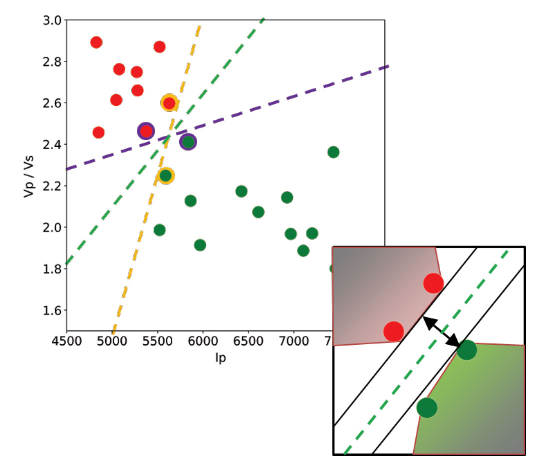
Let’s use a toy classification problem to understand in more detail how in practice SVMs achieve the class separation and find the hyperplane. In the figure below I show an idealized version (with far fewer points) of a Vp/Vs ratio versus P-impedance crossplot from Amato del Monte (2017, Seismic rock physics, tutorial on The Leading Edge).  I’ve added three possible boundaries (dashed lines) separating the two classes.

Each boundary is valid, but are they equally good? Well, for the SVM classifier, they are not because the classifier looks for the boundary with the largest distance from the nearest point in either of the classes.

These points, called Support Vectors, are the most representative of each class, and typically the most difficult to classify. They are also the only ones that matter; if a Support Vector is moved, the boundary will also move. However, if any other point is moved, provided that it is not moved into the margin or across the boundary, it would have no effect on the boundary. This makes SVM classifiers insensitive to outliers (points very far away from the rest of the points in their class and from the boundary) and also less memory intensive than other classifiers (for example, the perceptron). The process of finding this boundary is referred to as “maximizing the margin”, where the margin is a corridor with no data points between the boundary and the support vectors. The larger this buffer, the lower the generalization error; conversely, small margins are almost invariably associated with over-fitting. We will see more on this in a subsequent section.

So, to go back to the question, which of the three proposed boundaries is the best one (and by “best” I am referring to the one that will generalize better to unseen data)? Based on what we’ve learned so far, it would have to be the green boundary. Indeed, the orange one is so close to its support vectors (the two points circled with orange) that it leaves virtually no margin; the purple boundary is slightly better (the support vectors are the points circled with purple) but its margin is still quite small compared to the green boundary.

Maximizing the margin is the goal of the SVM classifier, and it is a constrained optimization problem. I refer interested readers to Hearst (1998, Support Vector Machines, IEEE Intelligent Systems); however, I will quote a definition from that paper (with reference to Figure 1 and accompanying text) as it yields further understanding: “… the optimal hyper-plane is orthogonal to the shortest line connecting the convex hulls of the two classes, and intersects it half way”.

In the inset in the figure, I zoomed closer to the 4 points near the green boundary; I’ve also drawn the convex hulls for the classes, the margin, and the shortest orthogonal line, which is bisected by the hyper-plane. I have selected (by hand) the best hyper-plane already (the green one), but if you can imagine rotating a line to span all possible orientations in the empty space close to the two classes without intersecting either of the hulls and find the one with the largest margin, you’ve just done quadratic optimization in your head. Moreover, you’ve turned a crossplot into a decision surface (quoted from Sebastian Thrun,  Intro to Machine Learning, Udacity 120 course).

If you are interested in learning more about Support Vector Machines in an intuitive way, and then how to try classification in practice (using Python and the Scikit-learn library), read the full article here, check the GitHub repo, then read How good is what? (blog post by Evan Bianco of Agile Scientific) for an example and DIY evaluation of  classifier performance.

What is acquisition footprint noise in seismic data?

Acquisition footprint is a noise field that appears on 3D seismic amplitude slices or horizons as an interwoven linear crosshatching parallel to the source line and receiver line directions. It is for the most part an expression of inadequate acquisition geometry, resulting in insufficient sampling of the seismic wave field (aliasing) and irregularities in the offset and azimuth distribution, particularly in the cross line direction.

Sometimes source-generated noise and incorrect processing (for example residual NMO due to erroneous velocity picks, incomplete migration, or other systematic errors) can accentuate the footprint.

This noise can interfere with the mapping of stratigraphic features and fault patterns, posing a challenge to seismic interpreters working in both exploration and development settings.

To demonstrate the relevance of the phenomenon I show below a gallery of examples from the literature of severe footprint in land data: an amplitude time slice (Figure 1a) and a vertical section (Figure 1b) from a Saudi Arabian case study, some seismic attributes (Figures 2, 3, 4, and 5), and also some modeled streamer data (Figure 6).

Bannagi combo

Figure 1. Amplitude time slice (top, time = 0.44 s) showing footprint in both inline and crossline direction, and amplitude section (bottom) highlighting the effect in the vertical direction. From Al-Bannagi et al. Copyrighted material.

Penobscop_sobel

Figure 2. Edge detection (Sobel filter) on the Penobscot 3D horizon (average time ~= 0.98 s) displaying N-S footprint. From Hall.

F3_shallow_sobel

Figure 3. Edge detection (Sobel filter) on a shallow horizon (average time ~= 0.44 s)  from the F3 Netherlands 3D survey displaying E-W footprint.

Davogustto and Marfurt

Figure 4. Similarity attribute (top , time = 0.6 s), and most positive curvature (bottom, time = 1.3 s), both showing footprint. From Davogustto and Marfurt. Copyrighted material.

Chopra-Larsen

Figure 5. Amplitude time slice (top, time = 1.32 s) the corresponding  coherence section  (bottom) both showing footprint. From Chopra and Larsen. Copyrighted material.

Long et al

Figure 6. Acquisition footprint in the form of low fold striation due to dip streamer acquisition. From Long et al. Copyrighted material.

In my next post I will review (with more examples form literature) some strategies available to either prevent or minimize the footprint with better acquisition parameters and modeling of the stack response; I will also discuss some ways the footprint can be attenuated after the acquisition of the data (with bin regularization/interpolation, dip-steered median filters, and kx ky filters, from simple low-pass to more sophisticated ones) when the above mentioned strategies are not available, due to time/cost constraint or because the interpreter is working with legacy data.

In subsequent posts I will illustrate a workflow to model synthetic acquisition footprint using Python, and how to automatically remove it in the Fourier domain with frequency filters, and then how to remove it from real data.

References

Al-Bannagi et al. 2005 – Acquisition footprint suppression via the truncated SVD technique: Case studies from Saudi Arabia: The Leading Edge, SEG, 24, 832– 834.

Chopra and Larsen,  2000 – Acquisition Footprint, Its Detection and Removal: CSEG Recorder, 25 (8).

Davogusto and Martfurt, 2011 – Footprint Suppression Applied to Legacy Seismic Data Volumes: 31st Annual GCSSEPM Foundation Bob F Perkins Research Conference 2011.

F3 Netherlands open access 3D:  info on SEG Wiki

Hall, 2014 –  Sobel filtering horizons (open source Jupyter Notebook on GitHub).

Long et al., 2004 – On the issue of strike or dip streamer shooting for 3D multi-streamer acquisition: Exploration Geophysics, 35(2), 105-110.

Penobscot open access 3D:  info on SEG Wiki

Computer vision in geoscience: recover seismic data from images, introduction

In a recent post titled Unweaving the rainbow, Matt Hall described our joint attempt (partly successful) to create a Python tool to enable recovery of digital data from any pseudo-colour scientific image (and a seismic section in particular, like the one in Figure 1), without any prior knowledge of the colormap.

Seismic picture on wall

Figure 1. Test image: a photo of a distorted seismic section on my wall.

Please check our GitHub repository for the code and slides and watch Matt’s talk (very insightful and very entertaining) from the 2017 Calgary Geoconvention below:

In the next two post, coming up shortly, I will describe in greater detail my contribution to the project, which focused on developing a computer vision pipeline to automatically detect  where the seismic section is located in the image, rectify any distortions that might be present, and remove all sorts of annotations and trivia around and inside the section. The full workflow is included below (with sections I-VI developed to date):

  • I – Image preparation, enhancement:
    1. Convert to gray scale
    2. Optional: smooth or blur to remove high frequency noise
    3. Enhance contrast
  • II – Find seismic section:
    1. Convert to binary with adaptive or other threshold method
    2. Find and retain only largest object in binary image
    3. Fill its holes
    4. Apply opening and dilation to remove minutiae (tick marks and labels)
  • III – Define rectification transformation
    1. Detect contour of largest object find in (2). This should be the seismic section.
    2. Approximate contour with polygon with enough tolerance to ensure it has 4 sides only
    3. Sort polygon corners using angle from centroid
    4. Define new rectangular image using length of largest long and largest short sides of initial contour
    5. Estimate and output transformation to warp polygon to rectangle
  • IV – Warp using transformation
  • V – Blanking annotations inside seismic section (if rectangular):
    1. Start with output of (4)
    2. Pre-process and apply canny filter
    3. Find contours in the canny filter smaller than input size
    4. Sort contours (by shape and angular relationships or diagonal lengths)
    5. Loop over contours:
      1. Approximate contour
      2. If approximation has 4 points AND the 4 semi-diagonals are of same length: fill contour and add to mask
  • VI – Use mask to remove text inside rectangle in the input and blank (NaN) the whole rectangle. 
  • VII – Optional: tools to remove arrows and circles/ellipses:
    1. For arrows – contours from (4) find ones with 7 sizes and low convexity (concave) or alternatively Harris corner and count 7 corners, or template matching
    2. For ellipses – template matching or regionprops
  • VIII – Optional FFT filters to remove timing lines and vertical lines

You can download from GitHub all the tools for the automated workflow (parts I-VI) in the module mycarta.py, as well as an example Jupyter Notebook showing how to run it.

The first post focuses on the image pre-processing and enhancement, and the detection of the seismic line (sections I and II, in green); the second one deals with the rectification of the seismic (sections IV to V, in blue). They are not meant as full tutorials, rather as a pictorial road map to (partial) success, but key Python code snippets will be included and discussed.

52 Things You Should Know About Geophysics

Matt Hall and Evan Bianco of Agile Geoscience have put together this great new book. I have been fortunate to have my article on colourmaps included as one of the 52 essays in the book. You can order the book directly from Agile’s publishing company Agile Libre:

52things

or you can order it on Amazon. For a look inside it, check here!